An Oldie, but a Goodie...Field Testing Frame Differences with a Power Meter

I originally posted this back in 2008 on the Slowtwitch.com forum and is an example of the types of equipment differences that can be determined with careful field testing.  Here's the link (click on the title below) to the full thread on Slowtwitch...it's long but informative, and there's some pretty good "back and forth" with a few skeptics:

Something Borrowed...Something Fast!

 
So take this guy and his position:

...and put him on this guy's bike and adjust it so that they fit identical.

Then, let the first guy test both of these "back to back" using the same 404 wheelset with PT SL hub and cover....Any guesses on what the aerodynamic drag differences (if any) one would see?

Using RChung's most excellent methodology described here: Method to the madness

Here's the results for the P2K with the 404 wheels (the wheels on the P3C above):

And here's the results for the P3C:

So...what's the bottom line?

Well...taking the same rider, the same wheels, the same basebars and brake levers, and with the seat and extensions adjusted to deliver the same positions...at basically zero yaw conditions I apparently measured a drag difference of ~.023 m^2 of CxA (or Cda, whichever you prefer - .228 m^2 for the P2K and .205 for the P3C). Using Doc C's "rule of thumb", that basically equates to ~2.5s per km of time savings.

With only an extremely small amount of crosswind however (I could just barely detect it on my skin, not enough to even move leaves on trees), the drag on both setups drops significantly, with the P3C setup dropping more at .190 m^2 vs. the P2K's .220 m^2 for a growing difference of ~.03 m^2. That translates to a difference of ~3 seconds per km...or a full 2 minutes over 40K.

Can you imagine comparing the difference between a P3C (or even the P2K) against a frame that actually increases in CxA with increasing yaw, which is actually fairly common?

Aero Field Testing using the "Chung Method" - How sensitive can it be?

As some of you may know, I've been field testing bike stuff and positioning with a power meter for 4 or 5 years now.  My method of choice is Robert Chung's "Virtual Elevation", or VE protocol, sometimes known as the "Chung Method".  He has a great presentation on it here: http://anonymous.coward.free.fr/wattage/cda/indirect-cda.pdf . When I first read Robert's info, I wrote up a spreadsheet that I've used since then to analyze everything from position changes to tire air pressure effects. Of course, since I wrote that spreadsheet for my own use, it's not exactly the most "user friendly" (Hey, I know what I'm supposed to do, I wrote it! ;-)...but, don't worry, everyone else is in luck since Andy Froncioni (the main tech guy behind Alphamantis and the ERO facility that recently opened at the indoor track in Carson) added a version of the same calculations (called "Aerolab") to the freeware power meter analysis software, Golden Cheetah.

So, the question with this type of testing usually comes down to just how sensitive can it really be...especially as compared to something like a wind tunnel?  Admittedly, there are some limitations to this type of testing, the main one being (at present time) that the results are mostly limited to zero yaw conditions, but as we saw in one of my previous blog posts, the most common yaw angles a TT'er or triathlete encounters are usually centered around zero yaw.  Using the tool to make evaluations at zero yaw still can hold a significant benefit for someone interested in improving/testing bicycle aerodynamics.

A couple years ago, Dr. Andrew Coggan published a blog post titled "A Challenge to Cycling Aerodynamicists" in which he described a field test he undertook to take up something he coined the "Tom Compton Challenge".  In short, it's an effort using known geometric shapes to try to determine the "sensitivity" of the aerodynamic field testing method.

Well, last year I discovered that my preferred field testing venue for VE runs had suffered some "traffic rerouting" that had made it much less appealing for the purpose (part of that "discovery" occurred when Andy sent his test setup to me to try and the results from my first course were very mixed due to excess vehicle interference after the nearby roads had been modified).  So, I started scouting around for an alternative course and luckily found one that is much closer to my home (I can ride there in just a few minutes) and that has laps that are significantly shorter than the old course (shorter laps = shorter test run time).  Both of these courses are best described as a sort of "extended halfpipe", an "out and back" course having a U-shaped elevation profile that allows for turnarounds to be taken at low speeds and thus avoid braking. Since identifying the new course, and having done just a few tests on it, one thing I wanted to do was to repeat the type of testing that Andy did and attempt to characterize the potential "sensitivity" of the course using the VE method.

Using Andy's setup as a guide, I set about figuring out what sorts of objects I could use for the test.  I took a quick trip to the nearby Michael's craft store and acquired some styrofoam spheres, 2", 3", and 4" in diameter.

In my garage I had an appropriate length of 1/2" diameter wooden dowel, and short work with a hand drill on the spheres and I had a setup that placed the spheres well out to the side where they should be in clear air while riding. Also shown in the pic above on the left is a small washer which I placed on the end of the dowel during the first run instead of a sphere.  I did that to act as a "cap" and make it more likely that the flow over the end of the cylinder stayed perpendicular.  Here's how the dowel and sphere setup looked after being zip-tied to the basebar of my TT bike.

The hole in each sphere ended up being a nice friction fit, so swapping between spheres was a very simple process. 

All runs were recorded with my trusty old yellow-cap PT Pro wheel mounted on the rear, with a cover in place to turn it into a de facto disc.  I prefer to use a PT for my aero field testing since it eliminates the uncertainty of variations in drivetrain resistance across the gearing, plus the PT's "coasting zero" feature allows me to have the power meter zero while soft-pedaling (i.e. turning the pedals slowly while freewheeling) down the descents of the course at least once per lap.  That helps to minimize any power meter drift during the runs.

So, with the test rig sorted out, it was time to head out to the test course and do some runs! To minimize wind and traffic effects, I prefer to head out to the course early on a Saturday or Sunday morning...before the small neighborhood that the course road services begins to wake up and starts moving around. A couple weekends ago, I headed out on a Sunday morning and rode over to my test course in 5 minutes, taking a small musette bag with the spheres, a notebook, and a couple of small tools I might need.  Starting at 6 am, I did the runs in the following order:

1. Rod only (w/washer "endplate")
2. 3" sphere
3. 2" sphere
4. 4" sphere

I mixed the runs up like that since I suspected that the "rod only" and 2" spheres may be close to the same measurement (part of the rod is covered up by the sphere) and I wanted to make sure there was a good separation between the cases.  I actually didn't sit down and calculate out the expected differences in CdA beforehand.  I wanted to first determine what the VE analysis showed as the differences from the baseline (run #1) and then see how close to the calculated values the VE runs were.  I did this because the method I use for determining the CdA using VE is a visual "leveling" procedure, and so there's a bit of "judgement" involved in determining what value best "fits" the overall plot to being level, and I didn't want that judgement being affected by any predetermined knowledge of what the expected differences should be.

Once I returned home, it was time to download the PT files into the computer and do the VE analysis.  As I described above, although it can be done in GC's Aerolab feature, I prefer to use my own home-brewed spreadsheet, mostly because I find it easier to expand the vertical scale to get a better handle on the leveling procedure, but also because I've recently added a feature that varies the on-road Crr as a function of the ambient temperature.  In order to use the spreadsheet, the following inputs are required:

1.  Total Mass - Easy to get just by stepping on a scale with bike in hand
2. Weather Conditions - this means air temp, dew point temp, and barometric pressure (to determine air density).  Luckily, there's a personal weather station listed on Weather Underground literally less than a block from my test course that has updates loaded every 5 minutes.  Using that station also allows for a cross-check on ambient wind conditions to make sure it stayed calm during the test runs.
3. Assumed Crr - For this, I use a weighted average of the front and rear tire Crr that I've determined from roller testing.  The spreadsheet then compensates for the expected Crr due to the difference in the test ambient temperature and the 20C temperature to which my Crr results are normalized.

As an example of the spreadsheet and what the VE profile plot ends up looking like, shown below is a snapshot of the first run from the testing:

OK then, let's get to the results.  Using the procedure outlined above, my best determination for the measured CdA from the runs was as follows (in order that runs were performed):

1. Rod only  = .2484 m^2
2. 3" sphere = .2498 m^2
3. 2" sphere = .2486 m^2
4. 4" sphere = .2510 m^2

Now, how does that compare to what should be expected for those shapes?  To determine that, I made a spreadsheet that calculated the expected CdA changes based on the typical values of Cd (in the Re number range of interest) for a sphere and a cylinder (sphere = 0.47, cylinder = 1.17) and their respective cross-sectional areas based on my actual measurements. As mentioned above, when I compared the "rod only" run to the sphere runs, I had to subtract the portion of the rod that was covered by the cylinder from the CdA calculation.  I then took those expected changes in CdA and added them to the measured CdA from the "rod only", or baseline run to determine the expected CdAs for the runs with the spheres.  Here's how they compared:

Run # - Sphere      Measured CdA (m^2)     Calculated CdA (m^2)   Difference (m^2)

2. - 3" sphere                  .2498                              .2501                          .0003
3. - 2" sphere                  .2486                              .2488                          .0002
4. - 4" sphere                  .2510                              .2518                          .0008


Another way of looking at it is the expected and measured differences from the baseline:

Run # - Sphere      Meas. Diff. from Baseline(m^2)     Calc. Diff. from Baseline (m^2)

2. - 3" sphere                       .0014                                            .0017
3. - 2" sphere                       .0002                                            .0004
4. - 4" sphere                       .0026                                            .0033


One last way of looking at this is from the perspective of expected change from from the previous run.  Here's how that worked out:

Run # - Sphere      Meas. Diff. from Previous (m^2)     Calc. Diff. from Previous (m^2)

2. - 3" sphere                       .0014                                            .0017
3. - 2" sphere                     -.0012                                           -.0013
4. - 4" sphere                       .0024                                            .0029

Not bad, huh?  I've always said that when using this technique I consider measurements that are within +/-.001 m^2 to be basically "tied", and the above appears to bear that assumption out as being fairly conservative.  It also gives me confidence that with careful technique I should be able to easily detect CdA differences on the order of .003-.005 m^2 and greater.

Tire Crr Testing on Rollers - The Chart..and a "how to"

In my last post I outlined the "math behind the madness" of testing the rolling resistance of bike tires on home rollers. In this one, I'll be showing the results of some of that testing I've personally done over the past year or so. I'll also go through a few tips and tricks I've learned in doing this sort of testing...just in case anyone else is crazy enough to try some of this potentially mind numbing testing.

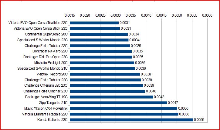
OK, I know a few of you are out there are "champing at the bit" to see the results, so without any further ado, here's a chart showing my estimates for the power to roll a pair of various tires I've tested (on a "real road" and for an 85kg bike plus rider mass):

Here's the same chart, but showing the estimated "on road" Crr values:

As can be seen, that's a fairly wide range of power requirements.  The wrong tire choice can easily "cost" a rider 10-15W of power to go a given speed.  When choosing tires, I commonly think of a scene from "Indiana Jones and the Last Crusade" where the Templar Knight guarding the Holy Grail says "...you must choose, but choose wisely...".  After all, when you're done with a race and you lose by seconds, or inches...you would hate to have the following be said about your tire choice:

The Setup:

OK, now that we've got that all out of the way, I thought I'd describe a bit about the setup I use for doing this sort of testing.  As you can see in the pic at the top of this blog post, it's a fairly simple affair consisting of a set of 4.5" diameter Kreitler rollers, a front fork stand, and a bike equipped with a power meter (and a power meter head unit).  That's really basically it.  A couple of other pieces of equipment that are crucial for getting consistent results, in my experience, are:

• A means to measure ambient temperature
• A means to measure rear wheel load
• A separate speed sensor and magnet (NOT on the wheel, but on the roller - see below)
• A notebook and pen

For measuring the ambient air temps during the test, I use my trusty Brunton ADC Summit, which I place at about axle level somewhere near the side of the rear wheel of the bike during the testing.

To measure the rear wheel load of the setup, I actually just use a digital bathroom scale which I've checked against known weights and typically is within 0.5 lbs of the actual weight.  In order to make that rear wheel load measurement, I mount the fork in the fork stand, and in stead of placing the rear wheel on the rollers, I stack the scale on top of some wood scraps and place the rear tire on the scale.  I stack it so that the rear axle is the same height off the ground as it would be on the rollers.  As it turns out, a couple of scrap pieces of 3" square wooden post and the thickness of my scale put that measurement to within 1/4" of what it is on the rollers.  Perfect.

Now then, let's talk about the speed sensor I mentioned above.  One of the most important things to get an accurate measure of in this testing is the actual "ground speed" during the test.  This can be done with a wheel mounted magnet and speed sensor, BUT that requires determining and changing the wheel rollout number for EACH tire tested.  In my experience, that can be a bit problematic...especially due to the curved contact patch that is present on the rollers.  It's very hard to get an accurate and consistent measure of wheel rollout that way.  To solve that problem, I realized that instead of triggering a speed sensor on the wheel, I could instead attach a magnet to the end of one of the rear drums and then use a speed sensor triggering off of the drum.  All I needed to do was to carefully measure the diameter of the metal drum (which will NOT be changing from test to test) and use THAT as the ground speed measurement for the testing.  Here's what that looks like:

That's just a small rare-earth magnet attached to the end cap of the roller with double-sided tape, and a Garmin ANT+ speed/cadence sensor taped to the roller frame.

Lastly, the notebook and pen are where I write down the date, what tire I'm testing, the size, the ambient temps during the testing, the power meter zero offset numbers, and the actual measured tire width as mounted.


The Protocol:

Alright, so everything is set up and we've gathered all the stuff needed.  What's next?  How do I do this? Well, here's a quick rundown of how I go about doing a tire Crr test (in "10 easy steps"!) This isn't the only way to do it, but it's how I've settled on things after doing this testing for a while:

1. Mount the tire on the test wheel - Most of my testing is done with my old yellow-cap PT wheel with a Mavic Open Pro rim.  I started out testing with this wheel in order to get both a hub and crank power to determine the level of typical drivetrain losses in the setup.  I wanted to know that for the occasions when I would be testing tires (such as tubulars) which I couldn't mount to the clincher PT wheel. Since I'm mainly interested in tires for time trials and road racing, I'll test them using a latex inner tube.  Testing by others has shown that using a butyl tube can cause 10-15% higher Crr than with latex.
2. Pump the tire to the test pressure - What pressure to use is really up to you.  I chose to do all of my testing with 120psi.  The reason I chose that value was mainly so that I could compare my results more easily to the results of others, most notably the testing done by Al Morrison.  Understand that on a perfectly smooth surface, the higher the pressure you pump tire up to, the lower the measured power requirements will be...however, that will only be true on the rollers, or on flat surfaces that are just as smooth.  On "real roads", i.e. roads with typical roughness, that isn't necessarily the case and there will tend to be a pressure above which higher pressures actually will make you slower overall.  Anyway, the key here is to pick a pressure and stick with it through your testing so that you are comparing tires on an equivalent basis.  
3. Place the wheel in the test bike - Install the rear wheel in the test bike and place the chain in the chosen gear for the testing.  I do my testing in a 53x13 gear for consistency. If it's not in there already, install the fork into the fork mount.
4. Measure the rear wheel load - This is done how I described above.  I'll usually only do this once during a session, and for me I've found it's typically within a pound or two each time (my body weight tends to be fairly stable).  This doesn't seem to be a super-critical measurement either, since a 1 or 2 lb. difference will only result in ~1-2% error in the final calculation.
5. Place rollers under rear wheel - At this point, move the scale out from under the rear wheel and slide in the rollers. To get a consistent placement of the rear wheel on the rollers, I'll lift the fork mount slightly off the ground while I allow the rear wheel to spin as it touches the 2 rollers and then I carefully place the fork mount on the ground.
6. Climb on board - It's now time to saddle up.  I usually approach the bike from the non-drive side and put my left foot on the pedal and then carefully swing my right leg over taking care not to disturb anything in the setup.  I'll then spin the cranks to make sure the PM is awake and the speed reading is working, at which point I'll clip out and zero the PM through the head unit.  I'll note the offset value (from my Quarq) in the notebook along with the ambient temperature.
7. Tire warmup - Now it's time to warm up the tire to working temperature.  Since my tests are done at 90 rpm (I find it's easier to hold a consistent rpm rather than focusing on the wheel speed) I'll warm up the tire at 95 rpm for 5 minutes.  At the end of the 5 minutes, I'll stop and quickly check the PM zero offset and write the value down in my notebook along with the ambient temperature reading.
8. The Test - Now it's time for the test.  I'll bring the cadence up to 90 rpms and once that is steady, I'll start a 4 minute interval in the PM head unit.  I'll concentrate on keeping a steady cadence through the whole interval, trying to be especially steady through the final 2 minutes since that is the section of the data I take the average power and ground speed from.  At the end of the 4 minute test interval, I'll again note the PM offset (to make sure it hasn't moved appreciably during the test for some reason) and write down the ambient test.  That's it.  Test over...either I stop there, or if I have more to tires to test, I'll start back at step one (skipping the load measurement for repeat tests) and on through the remaining steps.
9. Download Data - Now it's time to get the average power and ground speed values from the head unit.  I'll typically load the file into Golden Cheetah and then highlight the final 2 minutes of each test session and read off the averages as calculated.
10. Calculate the Crr - The final step is to take the average power and speed values, along with the wheel load and ambient temperature taken at the end of the test interval into a spreadsheet I've written to quickly do the calculations.  I've loaded the spreadsheet onto Google Drive and it can be accessed here: Crr Spreadsheet

Other Notes:

• After doing a number of runs using both the crank-based power meter and the PT wheel, I was consistently finding that for the gearing chosen and the lower power levels (typically 50-100W) seen on the 4.5" rollers, the drivetrain losses were on the order of 5%.  That's the value I enter in the spreadsheet.
• I did a fair number of runs with the exact same tire and at different ambient temperatures to determine what I should use as the temperature compensation value.  In my case, I found it to be ~1.36% change per deg C (lower Crr with higher temperatures).  Here's the plot of those tests:

• I normalize the Crr values to 20C.  If you want to know what the Crr would be at various temperatures, you can just enter those temperatures into the appropriate cell on the first sheet of the spreadsheet.
• Added 2/19/12 - I realized I forgot to point out that I use a "smooth to real road" factor of 1.5X to account for the higher energy dissipation requirements of typical road roughness.  This value is based on comparisons of roller based Crr measurements ("translated" to flat surface) and actual "on road" Crr derived from field tests and other means (i.e. iAero coast down values) for the same tires.

Well...that's about all I can think of for now.  Hopefully that will help encourage others to give this a try.  It's really not that difficult to do and is a good way to help you to "choose wisely" when it comes to tires for your "go fast" bike setup.

Tire Crr testing on Rollers - The Math

I've been doing a little bit of tire testing lately.  But, before I reveal any results, I thought it would be good to go over some math.  I know, I know...(I can hear the groans already), but I think it's important to review so people understand why it's reasonable to equate power to move a tire on a roller to power on flat ground.  

It's long been known that bicycle rollers act as a sort of rolling resistance "amplifier".  In other words, the differences in the rolling resistance between tires is magnified when riding on the rollers.  It's usually a fairly subtle thing to try to "feel" the difference in rolling resistance in tires when riding outside, but it's pretty easy to tell the fast tires from the slow tires on rollers just by the exaggerated effort it takes.  But, the question has long been "how much" of an amplifier are they? Well, back in 2006 I was discussing this with a few folks and realized that the equations to make that comparison between rollers and a flat surface Crr (Coefficient of rolling resistance) were already available...they just needed to be combined.  Then, it was pointed out to me that the particular geometry of a typical roller setup needed to be accounted for as well.  The normal "dual roller" setup on the rear of a roller set results in a geometric effect that actually increases the normal force on each roller.  In other words, you can't just take the rear wheel load as if it was a single roller. So, I added that to the equations as well.

Anyway, what you see below is the short "paper" I sketched up back then on the subject:

Flat Surface RR from Roller Testing – Tom Anhalt – 5/2/06

The power required to turn a wheel on a drum at a specific speed is governed by the equation:

P_Drum = Crr_Drum x V_Drum x M x g (a)

Where,

P_Drum = Power required to turn drum (Watts)

Crr_Drum = Coefficient of Rolling Resistance of the tire on the drum (unitless)

V_Drum = The tangential velocity of the drum (m/s)

M = The mass load of the wheel on the drum (kg)

g = gravitational constant = 9.81 m/s²

Rearranging equation (a) to solve for the Crr of the tire on the drum results in:

Crr_Drum = P_Drum / (V_Drum x M x g) (b)

Then the contact patch deformation of a tire of a specific diameter and a roller of a specific diameter can be equated to the deformation of an equivalent diameter tire on a flat surface using the following equation [Bicycling Science, 3^rd edition, pg 211]:

1/r_eq = 1/r₁ + 1/r₂ (c)

Where,

r_eq = equivalent wheel radius

r₁ = tested wheel radius

r₂ = tested drum radius

For convenience purposes, this equation can be rewritten using the appropriate diameters (r x 2) and is then:

1/D_eq = 1/D_wheel + 1/D_Drum (d)

For a tire of a given construction, it has been shown that the Crr varies inversely proportionally to the wheel radius, and thus the wheel diameter, in the range of D_wheel^0.66 to D_wheel^0.75 [Bicycling Science, 3^rd edition, pg. 226]. To simplify for this purpose, the assumption is made that the Crr varies inversely proportionally to D_wheel^0.7

From this, it can be then written that:

Crr_flat / Crr_Drum = D_eq^0.7 / D_wheel^0.7 (e)

Equation (e) can be combined with (d) and rearranged to give:

Crr_flat = Crr_Drum x [ 1 / (1 + D_wheel/D_Drum)]^0.7 (f)

Substituting equation (b) for Crr_Drum in equation (f) results in:

Crr_flat = [P_Drum / (V_Drum x M x g)] x [ 1 / (1 + D_wheel/D_Drum)]^0.7 (g)

Mass Correction Factor:

When doing Crr testing on rollers, the mass loading of the wheel or wheels will need to be corrected due to front-rear loading ratio and the fact that 2 offset rollers contact the rear wheel, thereby increasing the normal force on the rollers due to geometry effects.

Rear Wheel Only Case - When the test is done using a front fork mount and only the rear wheel contacting the rear rollers of the test setup, the following “effective mass” (M_eff) needs to be calculated and substituted for M in equation (g) :

M_eff = M_rear / cos [arcsin (X/(D_wheel + D_Drum))] (h)

Where:

X = separation distance of rear roller axles (consistent units with D_wheel and D_Drum)

M_rear = vertical mass load on rear wheel (kg)

Front and Rear Rollers - When the test is performed using both the front and rear rollers, the following Meff needs to be calculated and substituted for M in equation (g) :

M_eff = M_front + M_rear / cos [arcsin (X/(D_wheel + D_Drum))] (i)

Where:

M_front = vertical mass load on the front wheel (kg)

Power Correction:

Depending on the method of power measurement, the following offsets can be used to account for drivetrain and drum rotation losses in the calculation of P_Drum for use in equation (g):

For Powertap - P_Drum = P_Powertap – 5W (accounts for drum bearing losses) (j)

For SRM - P_Drum = P_SRM – 15W (accounts for drum bearings and driveline losses) (k)

Where:

P_Powertap and P_SRM are the power readouts (W) from the appropriate power meters.

These power offsets are somewhat arbitrary and should be modified if better data is known about the particular test setup.

That's basically it.  I'd like to note a couple things about the last section on "Power Correction".  First, after doing a bunch of testing since then, I don't bother accounting for the drum bearing losses.  Also, when using a crank-based power meter, like an SRM or a Quarq Cinqo, I've found (after using a PT in conjunction for quite a few tests) that it makes more sense to account for the drivetrain friction with just a straight percentage.  A typical value taken for drivetrain losses on bicycles is ~2.5%, but that is typical at higher power levels (i.e. higher chain tensions).  For the lower power levels I usually see in tire testing with a rear only roller setup (usually ~100W or less, with the better tires closer to ~50W) I typically see ~5% drivetrain losses, so that's the figure I use.

It's important to remember that the point of this is to get a "ballpark" feel for the difference between tires, not necessarily an absolutely accurate value.  It's been shown that percent difference in power requirements on the rollers equate very well to percent differences on the road.  What we're really looking for is a sort of "scaling factor" to put the differences seen on the rollers in perspective as to what to expect on the road.

There you go...equation (g) is easily written into a spreadsheet.  After that, it just takes a few measurements of the roller setup, weighing the rear wheel load, and some time on the rollers with a power meter equipped bike and nearly anyone can "test tires".

What's up with those funky rings...?

With the successes of Bradley Wiggins in 2012, there has been a lot of interest shown lately on the non-round rings he's been riding.  These rings are nothing new, and non-round rings have been dabbled with for a very long time, but the objective data (physical tests, as opposed to mathematical modeling) on whether or not these rings allow for a greater power output than round rings has been mostly in the negative.  Yet, there are typical reports of riders seeing 15-20W (or more) increases in their power output after mounting them on their bikes.  For a while, it's been speculated that some of these reports may be the result of an artificial inflation due to the way that some power meters calculate their power readings, and mathematical analyses along with user reports have suggested that the "real world" matches the artificial inflation theory.

What is this "artificial inflation" theory, you might ask?  Well, to understand the theory, first one has to understand how bicycle power meters measure and calculate power.  Simply put, for the most common power meters on the market (I'm talking SRM, Quarq, and PowerTap) there is a torque measurement that is averaged over a certain "window" that is then multiplied by the angular velocity to get power, i.e.

Power = Torque x Angular Velocity

However, the power output of a cyclist isn't constant torque, like with an electric motor, for example.  Instead, torque input to the crankarms of a bike is pulsed, with the majority of the torque being applied in a fairly narrow range during the pedal downstroke.  As such, if one plots torque vs. pedal position over a single pedal revolution, you'll typically see a sinusoidal-type plot with 2 "peaks" per pedal revolution.  Because of this, in order to better represent the true power output of a cyclist, the SRM and Quarq power meters have been designed to use what's known as an "event-based" power calculation algorithm.  What this means is that the torque is averaged over a complete pedal revolution (no matter how long it takes) and then the average torque is multiplied by the average angular velocity over that single pedal revolution.  This way, the only measure of angular velocity is a simple magnet/reed switch construction whereby each crank trigger signifies that 360 degrees of pedal rotation have been accomplished in the time between magnet pulses on the reed switch.  The over-riding assumption of this architecture is that the crank velocity does not vary significantly from the average during the pedal revolution, and with the high inertia of a cyclist traveling on the road at any reasonable speed, this is a fairly accurate assumption...with round rings that is.  If tension is maintained in the chain of the bicycle during the pedal stroke, then by definition the crank rotational velocity will be fairly steady.  If one where to be able to measure the instantaneous rotational velocity and the instantaneous torque and calculated the instantaneous power, then if you averaged all of those instantaneous power calculations over the complete pedal revolution, the result would be very close to averaging the torque over the complete pedal cycle and multiplying by the average rotational velocity.  This is why PMs have been designed this way.

Now then, how does this factor into non-round rings possibly causing artificially inflated power values?  Well, the way that most non-round rings are designed to "work" (one exception being the old Shimano Biopace rings) is that the effective chainring size is increased during the times that the legs are applying the highest amount of torque (and, since the system needs to be symmetric, also during the time when the leg is rising back into position in the "recovery" portion.  But, I digress..) and the effective chainring size is decreased during the portions of the pedal stroke across the top and bottom of the cycle. This causes the instantaneous rotational speed of the crank to vary in a roughly sinusoidal manner (dependent on the shape of the ring) above and below the average crank rotational velocity.

For a given wheel speed and for equivalent number of teeth on the chainring, the average rotational velocity of a non-round ring will be the same as for a round ring.  This is true because in order for the teeth to be at a spacing of 1/2", that means that the circumferences of a non-round and round ring of the same tooth count are equivalent.  However, with a non-round ring that means that, by design, the rotational velocity of the crank is being manipulated such that the rotational speed of the crank is slowed during the downstroke (and upstroke portions as well due to symmetry) to a value below the average

So, what does that mean?  In short, it means that during those times that the largest torques are being applied, the rotational velocity is lower than the average over the complete pedal revolution.  Since the majority of the power is produced in the downstroke portion of the pedal cycle, this means that power reported will tend to be over-reported, hence the term "artificial power inflation".  Get it?

So, that's the theory...how does it end up working in reality?  Well, in short, reality matches the theory fairly well and by my measurements, using Osymetric rings on a Quarq power meter will cause the Quarq to report a power value ~2.7-3.5% higher than reality.

Here's some testing I did near the end of 2012:

The setup: 

Test performed on a LeMond Revolution trainer to maintain a rear "wheel speed" similar to riding on the road (i.e. high flywheel inertia)
 
54T Round and 54T Osymetric both mounted on the same Quarq with the Osymetric in place of the inner ring. This was done to eliminate changes in drivetrain losses due to using different cogs. Calibration shows the Round ring (mounted on the outer position) reads 1% high and the Osymetric (mounted on the inner position) reads 1% low and the torque slope was set to the average value between the 2 rings. Power values from the Quarq reported below were corrected based on the calibration. Zero offset was checked before the first pair of runs, before the 2nd set of runs, and then at the finish. Offset did not move by more than 5 counts (512, 507, 511) which is equivalent to 1.3W @ 80 rpm. Runs were ~4 minutes in length.

Runs in order of performance:
- 54x15 gear, 80 rpm (36.2 km/hr indicated)

• Round Ring (Quarq - corrected) = 262.0W, LeMond Power Pilot = 249.5W, HR=160 bpm
• Osymetric    (Quarq - corrected) =271.3W, LeMond Power Pilot = 250.3W, HR=166 bpm

- 54x16 gear, 80 rpm (34.1 km/hr indicated)

• Osymetric  (Quarq - corrected) = 227.5W, LeMond Power Pilot = 212.3W, HR=158 bpm
• Round Ring (Quarq - corrected) =221.6W, LeMond Power Pilot = 212.0W, HR=161 bpm

So, in brief, based on just this limited test, there actually DOES appear to be a "non-round ring inflation factor" of 2.7%-3.5%. (BTW, Dan Connelly estimated a 4% "inflation" based on a 20% within pedal stroke speed variation here (http://djconnel.blogspot.com/...uniform-cadence.html) and by my measurements the Osymetric ring would cause a 20% crank speed variation assuming a constant rear wheel speed.

I followed up the trainer testing rides outside where I ran a PT wheel on the same bike as the Quarq/Osymetric setup with the large ring being the non-round ring and the small ring being round.  The artificial inflation with the non-round ring was observed there as well with the difference between the power as measured by the Quarq as compared to the PT being ~4% higher when in the non-round ring under a continous effort.
 
So, there you have it...my suspicion is that a good majority of the power "improvements" claimed with non-round rings are merely mis-measurements of the actual power.  It's important to note that this sort of power inflation is not anything that can be "calibrated out".  It will be present even if the PM torque calibration is perfect since it's a result of the power calculation algorithm itself and ANY power meter that employs an "event-based" calculation as described above will suffer from it.

Now then...on the question of whether or not non-round rings have the potential to actually increase pedaling power output...well, I have my opinions on that, but I'll leave that for another blog post....